Rates, Normalization and Consolidation

Statistics module stores rates during time intervals. These time intervals are on well defined boundaries in time. However, your input is not always a rate and will most likely not be on such boundaries. This means your input needs to be modified. This section explains how it works.

A couple of different stages should be recognized:

• transforming to a rate

• normalizing the interval

• consolidating intervals into a larger one

This does not get in your way, it is not doing bad things to your data. It is how SPC module works, by design.

All stages apply for all input, no exceptions. There is no short circuit. After transforming your input into a rate, normalization occurs. After normalization, consolidation occurs. All three stages can be a no-op if you carefully setup your database, but making one stage a no-op does not mean the other stages are skipped.

If you use Gauge, the input is already a rate, but it is still subject to normalization. If you enter the data exactly at the boundaries normalization is looking for, your input is still subject to consolidation.

Everything is processed as a rate. This doesn't mean you cannot work with temperatures, just remember it is processed as if it was a rate as well.

There are several ways for SPC module to get a rate from its input (depending on the channel type):

Gauge:

Keep it "as is". The input is already a rate. An example would be a speedometer. This is also the type used for keeping track of temperature and such.

Keep it "as-is" does not mean normalization and consolidation are skipped! Only this step is.

Counter:

Look at the difference between the previous value and the current value (the delta). An example would be an odometer. The rate is computed as: delta(counter) divided by delta(time).

Absolute:

As the odometer, but now the counter is reset every time it is read. Computed as: value divided by delta(time).

Derive:

As counter, but now it can also go back. An example could be something monitoring a bidirectional pump. The resulting rate can be negative as well as positive.

In each of these four cases, the result is a rate. This rate is valid between the previous update of statistical channel and the current one. SPC module does not need to know anything about the input anymore, it has start, end and rate.

This concludes step 1. The data is now a rate, no matter what data source type you use. From this moment on, SPC module doesn't know nor care what kind of data source type you use.

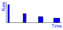
If you transfer something at 60 bytes per second during 1 second, you could transfer the same amount of data at 30 bytes per second during 2 seconds, or at 20 bytes per second during 3 seconds, or at 15 bytes per second during 4 seconds, et cetera.

These numbers are all different yet they have one thing in common: rate multiplied by time is a constant. In this picture, it is the surface that is important, not its width nor its height. This is because we look at the amount of data, not at its rate nor its time. Why this is important follows later.

The input is now a rate but it is not yet on well defined boundaries in time. This is where normalization kicks in. Suppose you are looking at a counter every minute. What do you know? You know counter values at HH:MM:SS. You don't know if the counter incremented at a high rate during a small amount of time (1 second at 60 bytes per second) or during a long time at a small rate (60 seconds at 1 byte per second). Look at the picture above again, each HH:MM:SS will be somewhere in the white areas.

This means that the rate you think you know isn't the real rate at all! In this example, you only know that you transferred 60 bytes in 60 seconds, somewhere between MM:SS and the next MM:SS. Its computed rate will be 1 byte per second during each interval of 60 seconds. Let me emphasize that: you do not know a real rate, only an approximation.

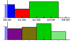
Now look at the next image, showing some measured intervals and rates. The samples are taken at 30 seconds past the minute, each colored area represents another measurement. There are four measured intervals, the last one has a rate of zero but it is known (i.e. the last update occurred at 04:30). One expected update, the one at 02:30, did not happen. SPC module can cope with this perfectly well if you let it. The update just happens at 03:30 and is valid from 01:30.

The bottom part of the image is the result after normalization. It shows that each interval uses a bit of each input interval. The first interval is built from the blue interval (which started before 00:00) and the red interval (measured between 00:30 and 01:30). Only the blue part that falls inside the 00:00 to 01:00 interval is used, only the red part that falls inside the 00:00 to 01:00 interval is used. Similar for the other intervals. Notice that it are areas that are important here. A well defined part of the blue area is used (in this example exactly half) and a well defined part of the red area is used (dito). Both represent bytes transferred during an interval. In this example we use half of each interval thus we get half of the amount of bytes transferred. The new interval, the one created in the normalization process, has a surface that is exactly the sum of those two amounts. Its time is known, this is a fixed amount of time, the step size you specified for your database. Its rate is its area divided by this amount of time.

If you think it isn't right to shift data around like this, think again. Look at the red interval. You know something has happened between 00:30 and 01:30. You know the amount of data transferred but you do not know when. It could be that all of it was transferred in the first half of that interval. It could also be that all of it was transferred in the last half of that interval. In both cases the real rate would be twice as high as you measured! It is perfectly reasonable to divide the transfer like we did. You still don't know if it is true or not. On the long term it doesn't make a difference, the data is transferred and we know about it.

The rates are now normalized. These are rates that statistics module works with. Notice that the second and fourth normalized rate (mixture of red and green, mixture of green and white) are lower than the green rate. This is important when you look at maximum rates seen. But as both the red and green rates are averages themselves, the mixture is as valid as its sources.

Each normalized rate is valid during a fixed amount of time. Together these are called Primary Data Points (PDPs). Each PDP is valid during the step size. SPC module doesn't know nor care about the input you gave it. This concludes step 2. From now on, SPC module forgets all original input.

Even if normalization is a no-op (if you made sure your timestamps are already on well defined boundaries) consolidation still applies.

Suppose you are going to present your data as an image. You want to see ten days of data in one graph. If each PDP is one minute wide, you need 10*24*60 PDPs (10 days of 24 hours of 60 minutes). 14400 PDPs is a lot, especially if your image is only going to be 360 pixels wide. There's one way to show your data and that is to take several PDPs together and display them as one pixel-column. In this case you need 40 PDPs at a time, for each of the 360 columns, to get a total of ten days. How to combine those 40 PDPs into one is called consolidation and it can be done in several ways:

Average:

Compute the average of each rate (of those 40)

Minimum:

Take the lowest rate seen (of those 40)

Maximum:

   Take the highest rate seen (of those 40)

Sum:

   Take the sum of those 40 rates

First:

   Take the first rate seen (of those 40)

Last:

   Take the last rate seen (of those 40)

Which function you are going to use depends on your goal. Sometimes you would like to see averages, so you can use it to look at the amount of data transferred. Sometimes you want to see maxima, to spot periods of congestion, et cetera.

Whichever function you use, it is going to take time to compute the results. 40 times 360 is not a lot but consider what's going to happen if you look at larger amounts of time (such as several years). It would mean you have to wait for the image to be generated.

This is also covered by SPC module but it requires some planning ahead. In this example, you are going to use 40 PDPs at a time. Other examples would use other amounts of PDPs each time but you can know up front what those amounts are going to be. Instead of doing the calculations at use-time, SPC module can do the computations at monitoring time. Each time a series of 40 PDPs is known, it consolidates them and stores them as a Consolidated Data Point (CDP). These are CPDs that are stored in the database. Even if no consolidation is required, you are going to "consolidate" one PDP into one CDP.

Was this page helpful?

Tell us more

Send

Thank you!