Making Predictions with the Machine Learning Module
As you continue to work with the Iotellect platform and develop your application, you may want to incorporate tools for data analysis and prediction. One useful tool is the Machine Learning module. The following example will show how to use a linear regression algorithm to create a model that predicts the relationship between an independent and dependent variable. In this case we will predict the amount of energy collected (dependent variable) based on the average daily luminescence (independent variable). By understanding this relationship, we can make more accurate predictions about future power generation and identify potential issues or opportunities for improvement. In this chapter of the tutorial, we will guide you through the process of using linear regression to create a model for predicting power generation based on luminescence data from the solar panel power station.
There are a number of different algorithms available through the Machine Learning module all of which follow a similar usage pattern. The following will take you through the basic process:
Preparing appropriate datasets
Creating data structures in Iotellect for machine learning tasks
Creating and configuring an Iotellect Trainable Unit
Training the Trainable Unit
Testing the Trained Unit
Generating Predictions from Trainable Units
Incorporating Predictions into Dashboards
Preparing Appropriate Datasets
In order to make predictions and accomplish other machine learning tasks like classification, we can train a mathematical model based on existing data. We will be making predictions based on daily historical luminescence values for the region where our power plant is located, and total energy generation for that day.
In the following example, the data is in a file with elements separated by semicolons. There are about 500 data points in the data set we are using. Our file looks something like the following:
luminescence;energy
0.267027698;32.54661902
0.976869989;55.39033824
3.664669577;71.16015301
3.986523168;131.6570175
4.236464973;118.8121496
4.865873622;188.1513313
...
etc
...The first concept to address splitting the data set into a training data set and control data set. The training data is what will be used to create the mathematical prediction model, and the control data is what we will use to test the accuracy of the model. The testing and training data needs to be different, otherwise we will not be able to identify when our model has been overfitted to the training data. We can say a model is overfitted when it corresponds too closely or exactly to a particular set of data.
We will be using the mathematically simple model of linear regression, where overfitting generally isn’t a problem unless there are not enough data points in relation to the parameters of the model. An in-depth discussion of the mathematics involved is outside the scope of this document, but in this example 500 data points are more than enough for a single prediction parameter.
Training Data
We randomly select 70% of the lines of our data set, creating a document with about 350 data points, formatted like the following:
luminescence;energy
0.267027698;32.54661902
0.976869989;55.39033824
3.664669577;71.16015301
... 350 more data pointsControl Data
The remaining 30% of the lines of our data set form a document with about 150 lines similar to the following:
luminescence;energy
3.986523168;131.6570175
4.236464973;118.8121496
4.865873622;188.151331
...150 more data pointsCreating Data Structures for Machine Learning Tasks
Now that we have training and control data sets, we need to create the correct data structures in Iotellect. From the context menu of the Models node in the System Tree, select Create.
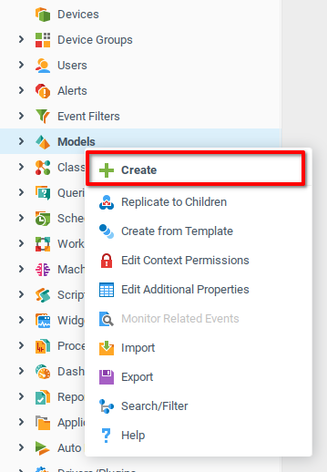
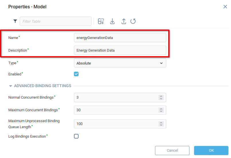
Add an appropriate Name and Description for the model, and click OK.
From the Model Configuration window which appears:
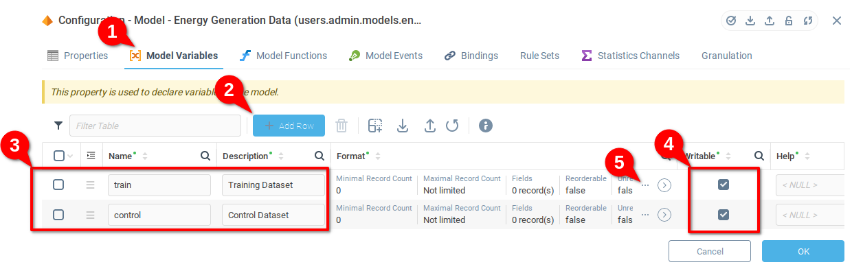
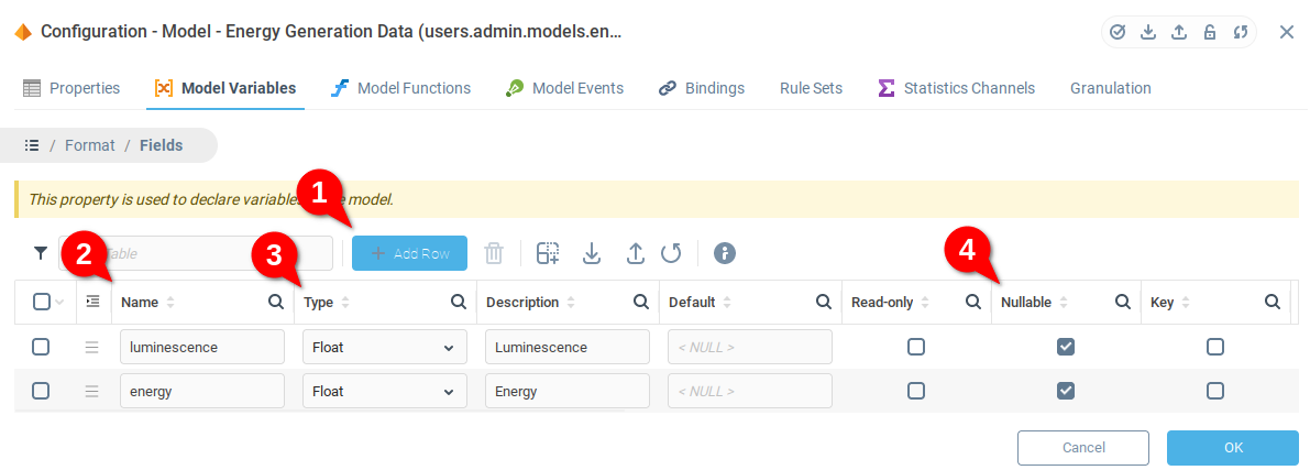
Select the Model Variables tab.
Add two rows to the table.
Add appropriate names and descriptions for the training and control datasets.
Set both variables to Writable.
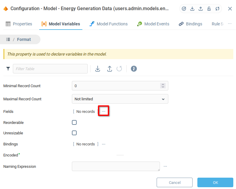
Open the details of the Format field (you need to do this for both variables)
From the Format details, open the Fields details
In the Fields list:
Add two fields.
Add an appropriate name (and description if desired).
Set the Type to Float for both fields.
Set the Nullable flag to allow both fields to take the value Null.
Once you have added Luminescence and Energy fields to the Train variable, repeat the preceding steps for the Control variable.
Once you’ve added Luminescence and Energy fields to the Control variable, save and close by pressing OK.
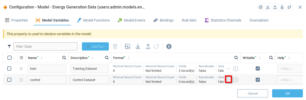
Loading Data Into the Model
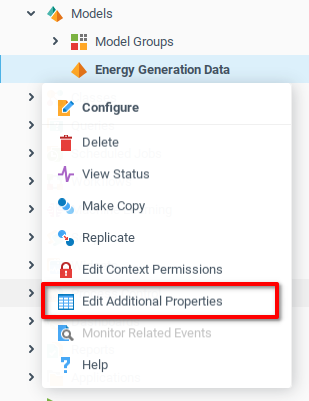
Now that the appropriate variables have been created in the model, choose Edit Additional Properties from the context menu of the model which you created in the previous step.
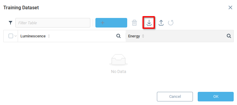
We see the variables created in the previous section, Control Dataset and Training Dataset. Unlock the variables for editing (1) and then open the Training Dataset (2).
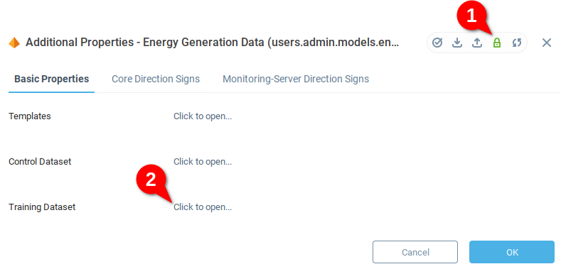
No data has been added, so the table is empty. Choose the import data icon import a file. Load the data for your training dataset.
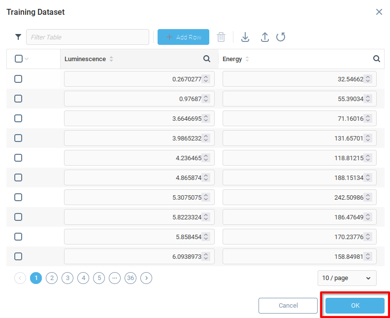
If the import is successful, the field should be populated with the training data. Click OK to save and close.
Repeat the above steps for the Control Dataset, ensuring that the correct data is loaded.
Creating and Configuring a Trainable Unit
Now that we have a model with the training and control data, the next step is to configure the Trainable Unit. The Trainable Unit is a child of the Machine Learning context, and every instance of a Trainable Unit represents one model using a specific algorithm and specific hyperparameters.
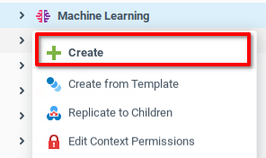
From the Machine Learning context, open the context menu and select Create.
From the Properties menu of the Trainable Unit,
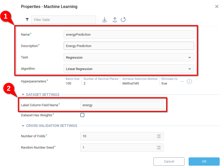
Add an appropriate Name and Description, selecting Regression and Linear Regression respectively for Task and Algorithm.
Indicate the name of the variable you want to predict, In the case of the example, we want to predict the amount of energy generated based on the amount of luminescence. When we send data to the model for training, testing, or generating predictions, there must be a column with the name
energy, otherwise the unit will return an error. The model created in the previous step has columns namedluminescenceandenergy.
Click OK to save and close. Our Trainable Unit is now ready to be trained.
Training and Testing the Trainable Unit
In order to train and test the Trainable Unit which we created in the previous section, we need to create to call the “train” and “evaluate” functions of the unit. First we will create model functions in the Energy Generation Data model to show how the Expression Language can be used to use the a trainable unit.
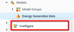
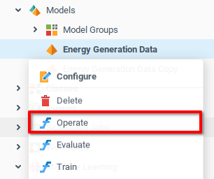
Open the Configure option from the Energy Generation Data model context menu.
From Configuration menu of the Energy Generation Data model:
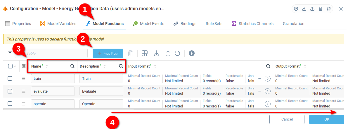
Navigate to the Model Function tab.
Add three rows to the function table.
Add Names and Descriptions to the functions. The example below uses
train,evaluate, andoperatefor the three functions.Scroll right to find the Expression field.
The Expression field of the function allows us to define an expression which will be called when the model function is called. We use the model functions for the purpose of demonstration, but in principle you can use the callFunction() of Context-Related Functions from any expression in Iotellect. This allows you to fully automate usage of the Trainable Units.
From the Model Functions tab, now scrolled to the right, you can see the Expression field for each of the functions. Below we describe the expressions to add to each row.
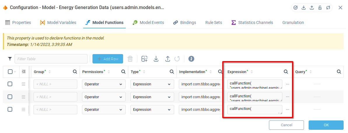
As mentioned above, we will use the Expression Language function callFunction() of Context-Related Functions in order to use functions of the Trainable Unit. The first two parameters of callFunction() are the context path from which we want to call the function, and the name of the function. The remaining parameters are determined by the function being called. In the case of the three functions of the Trainable Unit, the only remaining parameter is the data table with training, evaluation, or operation data.
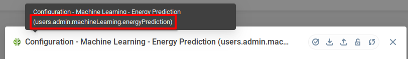
Mouse over the Configuration window of the Trainable Unit to find the Context Path. We find the context path users.admin.machineLearning.energyPrediction for our Trainable Unit.
The next parameter of callFunction() is the name of the function we want to call. From the Trainable Unit documentation, we know there are three functions to use, train in order to train the model, evaluate to get some statistics to see if the model performs with the necessary accuracy, and operate when we want to make actual predictions with the model.
Finally, the question is where we are going to take the data from. Recalling that we named the variables in the model train and control, and knowing that the context path for the model is users.admin.machineLearning.energyPrediction, we can create a path to the variable with the : operator and enclose the result in {} brackets.
To access the training data, we will use {users.admin.models.energyGenerationData:train} and the control data {users.admin.models.energyGenerationData:control}. Putting these elements together, we are provided with the following expressions to put in the Expression field of the model functions:
Train
callFunction(
  "users.admin.machineLearning.energyPrediction",
  "train",
  {users.admin.models.energyGenerationData:train}
)Evaluate
callFunction(
  "users.admin.machineLearning.energyPrediction",
  "evaluate",
  {users.admin.models.energyGenerationData:control}
)Operate
callFunction(
  "users.admin.machineLearning.energyPrediction",
  "operate",
  {users.admin.models.energyGenerationData:control}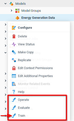
)Now that the functions are in place, we can call them from the context menu of the Energy Generation Data model. First train the model by calling the Train function. and confirming the subsequent confirmation dialogue.
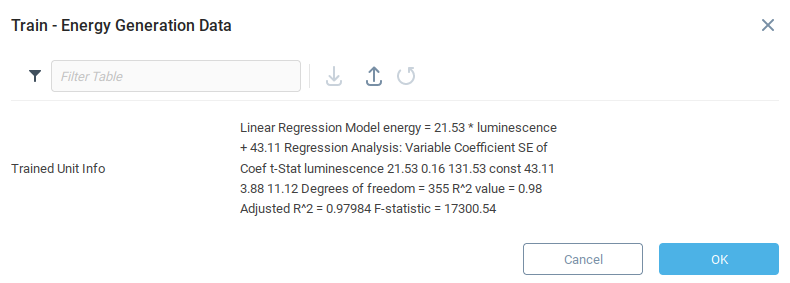
Having trained the model, we are presented with some data related to the accuracy of the model. Since we are using a linear regression, the model presents the exact formula generated from running the regression against the training data. Each model will return information specific to the algorithm used.
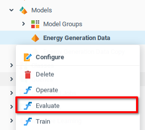
Now that we have trained the model, we can test it for accuracy. Again open the Energy Generation Data model context menu, but now select the Evaluate function, and confirm the operation.
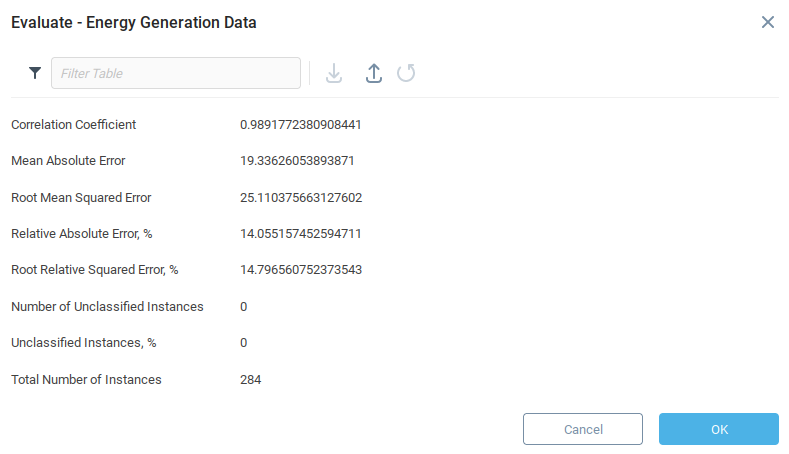
The evaluate function of the Trainable Unit produces a number of metrics related to the accuracy of the model.
Now that the model is trained and we’re satisfied that the initial error metrics are correct, we can use the model for making predictions.
Getting Predictions from Trainable Units
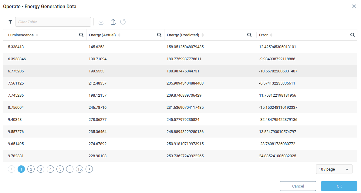
Making predictions from a Trainable Unit requires data in the same format as the training data. In the example we’re using, for now we make predictions using the control data because it already has the correct format. Call the Operate function from the Energy Generation Data model context menu.
The operate function takes the provided data and generates predictions using the model, compares predictions to the actual values and displays error values. Since we used the control data, there is already an “Actual” value. In practice, the “Actual” value will be set to zero.
Exploring Further
Now that you have a broad understanding of how to use Trainable Units, you may consider:
Adding this information to a dashboard chart.
Explore using different algorithms for trainable units.
Was this page helpful?